Geometric Deep Learning for Wireless Communication Networks

Under Professor Bruno Clerckx and Matteo Nerini, I am currently undertaking a research project on the application of Geometric Deep Learning on the power allocation problem in MIMO wireless communication channels (referred to as a K-user interference channel). This research is based on the paper: Graph Neural Networks for Scalable Radio Resource Management: Architecture Design and Theoretical Analysis by Yifei Shen, Yuanming Shi, Jun Zhang, and Khaled B. Letaief. The primary codebase for this research can be found in https://github.com/yshenaw/GNN-Resource-Management. The current aim is to improve the results of the work presented in the research through network tuning and supervised learning (instead of the unsupervised method used in the paper).

Wireless communication channels suffer from considerable interference between transmitter-receiver pairs, measured by the metric SINR (Signal-to-interference plus noise ratio). The goal in the wireless communication network is thus to maximize the SINR for every transmitter-receiver pair, e.g. by increasing the power (bound by some max power P_max). However, increasing the power of any one transmitter-receiver pair increases the intereference power to other nearby channels, the level of interference of which depends on whether it utilizes a beamforming array or a conventional (radial) array. Therefore, this problem is a non-convex optimization problem.

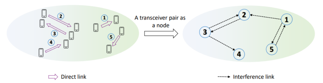
The transmitter-receiver pair in our network can be represented as nodes of a graph data structure. The node in itself contains important information, such as the pair's weight in the network, as well as the channel state. Each edge between nodes represent interference between transmitter-receiver pairs. Observe the diagram below:

The node features of node k can be denoted as h_k,k, w_k, and σ_k², whilst the edge features (representing interference) between node j and node k is denoted by h_j,k. From this representation, we can denote the SINR as:

$$SINR_k = {|h_{k,k}^{H}v_{k}|^2 \over \sum_{j \neq k}^{K}|h_{j,k}^{H}v_{j}|^2 + \sigma_k^2}$$

Given a certain beamforming matrix V, the objective is thus to find the optimal beamformer design to maximize the average sum rate in the network. This is given by the optimization formulation below: $$\underset{V}{maximize} \; \sum_{k=1}^{K}w_klog_2(1+SINR_k)$$ $$subject\;to \; ||v_k||^2_2 \leq P_{max}, \forall k$$

Many existing algorithms used for power allocation problem uses a convex optimization approach to solve this non-convex optimization problem, and are thus limited in both performance and scalability. A classical example include the WMMSE (weighted minimum mean-square-error). An alternative solution is thus to use a Graph Neural Network (GNN) (also referred in the paper as the WCGCN - wireless channel graph convolution network), a powerful emerging type of neural network used in extracting non-linear relationships between nodes in a graph through a process known as node aggregation and message passing. A powerful advantage of using neural networks for this optimization is its much smaller computation time. Unlike WMMSE, where for each channel realization we have to run a lengthy optimization algorithm, neural networks - after it has been trained - can immediately compute the power allocation without using any iterative algorithm by simply passing the input through the trained neuron weights. The speed of this can be further accelerated through the use of modern GPUs. An illustration of a graph neural network is shown below:

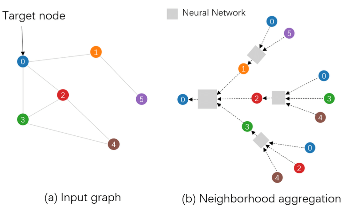
Each gray box is a non-linear node aggregator, typically a deep neural network. This neural network is trained similarly to that of vanilla neural networks through backpropagation of a loss (given by some loss function) and performing an optimization step (e.g. gradient descent). Graph neural networks are extremely powerful in this application, not only due its effectiveness against overfitting (i.e. it works well even with low training data), but also its generalizability. If new nodes enter or leave the network, the GNN will still function well and does not need to be re-trained.

In the research paper, the negative sum rate is used as a metric for the loss function of our neural network. Recall that our goal is to maximize the sum rate, thus by allocating power such that we minimize the negative sum rate, we are effectively maximizing the sum rate. This is formulated below:

The loss function above defines an unsupervised method of training our GNN, as we require no pre-defined node labels (or ground truth power allocation) to train against; instead, the neural net tries to come up with the power allocation which minimizes the loss function directly.

However, while the finding in the research has proven extremely effective - i.e. the neural network computation time is orders of magnitude smaller than traditional optimization algorithms, the performance of the WCGCN more or less matches (or is slightly suboptimal to) the traditional WMMSE algorithm. The research that I am conducting, therefore, looks at how to improve the performance of the WCGCN architecture defined in the research paper, particularly through a potentially supervised approach. One idea is to use the 100x WMMSE algorithm, which runs the WMMSE optimization algorithm 100 times with randomized initialization, and choosing the power allocation which obtains the highest sum rate. The resulting sum rate of this algorithm is typically around 10% to 15% higher than the WCGCN approach; however, it is much, much slower. Thus, by computing the 100x WMMSE algorithm as the ground-truth power allocation values and training the WCGCN in a supervised approach, we can potentially get the higher performance of the 100x WMMSE, whilst also retaining the extremely fast computation speed of the WCGCN.